Learning about Microsoft Excel functions related to cell in get cell value by address [1], find the last non-empty cell [2], return a reference to a range [3], create cell address [4].
Returns a value or reference of the cell at the intersection of a particular row and column,in a given range. Format INDEX(array, row_num, [col_num]), where array is something like 'Sheet'!A1:C4, and row_num and col_num are simply a number. Following
=INDEX('MyData'!C3:F5, 2, 3)
will give the value of cell with address E4 in the sheet with name MyData.
Looks up a value either from a one-row or one-column range or from an array. Provided for backward compatibility. Format LOOKUP(lookup_value, lookup_vector, [result_vector]), where look_value is the value to be found, but when it can not be found then it will match the next smallest value, lookup_vector is a vector with values to be examined, and result_vector is a vector with component to be displayed. Then
=LOOKUP(2, 1/('MyData'!K:K <> ""), 'MyData'!L:L)
will give find the last non-empty row of colum K:K and use it to show the corrresponding row in column L:L. It is not necessary to use 'MyData' when refering cell in the same sheet. The ('MyData'!K:K <> "") will create array of true and false which will be treated as 1 and 0 when operated through 1/('MyData'!K:K <> "").
Returns the reference specified by a text string. Format =INDIRECT(ref_text, [a1]) will convert the ref_text into a reference with “A1” style if second argument is true or “R1C1” style if it is false.
=INDIRECT("B4")
will give value of cell with address B4.
Creates a cell reference as text, given specified row and column numbers. Format =ADDRESS(row_num, column_num, [abs_num], [a1], [sheet_text]). Then following functions
=ADDRESS(2,3,1)
=ADDRESS(2,3,2)
=ADDRESS(2,3,3)
=ADDRESS(2,3,4)
will give
$C$2
C$2
$C2
C2
respectively, as cell references.
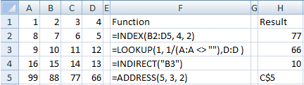
Following image shows the use of INDEX, LOOKUP, INDIRECT, and ADDRESS functions.
Please refer to previous section for detail of each function.