Copyright © 2018 John Wiley & Sons, Inc. and primarily advanced by Prof. A. Iskandar.
A Message from Prof. Michio Kaku Link to heading
url https://www.youtube.com/watch?v=weVBAQhl804
We physicists flunk students taking elementary physics. And more or less encouraged to do so by engineering department.
We don’t want to train engineer who makes bridges that fall down. Engineers that create skyscrapers that fall over.
And you encounter freshment physics for the first time, watch out. If you have a rough time, that’s the way it is.
Kaku was inspired to pursue a career in physics after seeing a photograph of Albert Einstein’s desk at the time of his death.
Kaku was fascinated to learn that Einstein had been unable to complete his unified field theory and resolved to dedicate his life to solving this theory.
By the time Kaku was in high school, he had developed a strong passion for physics, then for a science fair, Michio built a 2.3 MeV “atom smasher” in his parents’ garage.
Elon Musk’s obsession with truth Link to heading
url https://www.youtube.com/watch?v=Tu4DaH2MIg4
So for me, physics was sort of a very natural thing to study.
Nobody made me study.
Menteri Kesehatan RI Link to heading
url https://www.youtube.com/watch?v=vfKIP0u2q-g&t=15s
.. sebagai asalah satu alumni Prodi Fisika, Fakultas MIPA, Institut Teknologi Bandung ..
.. saya mendapatkan banyak kesempatan untuk mengembangkan kemampuan diri, baik secara keilmuan fisika itu sendiri, maupun kemampuan-kemampuan lain yang berguna bagi kelanjutan karir saya.
Untuk adik-adik saya tercinta, mahasiswa fisika ITB, baik yang baru saja lulus maupun yang sedang menjalani pendidikan, ambilah semua kesempatan-kesempatan yang ditawarkan oleh Jurusan Fisika ITB, dalam pengalaman ilmu untuk menuju karir yang berkualitas serta membangun bangsa dan negara ke arah yang lebih baik.
Dan untuk Anda yang bercita-cita berkuliah di Fisika ITB, yakin dan bersiaplah untuk menempuh jalan yang berliku dan penuh makna.
Kejarlah keinginanmu tanpa ragu dan persiapkan masa depanmu semaksimal mungkin.
2-1 Position, Displacement, and Average Velocity (1 of 9) Link to heading
Learning Objectives
- 2.01 Identify that if all parts of an object move in the same direction at the same rate, we can treat it as a (point-like) particle.
- 2.02 Identify that the position of a particle is its location on a scaled axis.
- 2.03 Apply the relationship between a particle’s displacement and its initial and final positions.
- 2.04 Apply the relationship between a particle’s average velocity, its displacement, and the time interval.
- 2.05 Apply the relationship between a particle’s average speed, the total distance it moves, and the time interval.
- 2.06 Given a graph of a particle’s position versus time, determine the average velocity between two times.
2-1 Position, Displacement, and Average Velocity (2 of 9) Link to heading
- Kinematics is the classification and comparison of motions
- For this chapter, we restrict motion in three ways:
- We consider motion along a straight line only
- We discuss only the motion itself, not the forces that cause it
- We consider the moving object to be a particle
- A particle is either:
- A point-like object (such as an electron)
- Or an object that moves such that each part travels in the same direction at the same rate (no rotation or stretching)
2-1 Position, Displacement, and Average Velocity (3 of 9) Link to heading
- Position is measured relative to a reference point:
- The origin, or zero point, of an axis
- Position has a sign:
- Positive direction is in the direction of increasing numbers
- Negative direction is opposite the positive
Gambar garis bilangan dilengkapi di bagian atas dengan panah arah ke kanan menggambarkan arah positif dan di bawahnya panah arah ke kiri menggambaarkan arah negatif, origin terletak di titik 0, satuan garis bilangan dalam m, $x \in [-3, 3]$.
Figure 2-1
2-1 Position, Displacement, and Average Velocity (4 of 9) Link to heading
- A change in position is called displacement
- $\Delta x$ is the change in $x$, (final position) − (initial position) $$\tag{2-1} \Delta x = x_2 - x_1 $$
- Examples A particle moves . . .
- From x = 5 m to x = 12 m: $\Delta x = 7$ m (positive direction)
- From x = 5 m to x = 1 m: $\Delta x = -4$ m (negative direction)
- From x = 5 m to x = 200 m to x = 5 m: $\Delta x = 0$ m.
- The actual distance covered is irrelevant
2-1 Position, Displacement, and Average Velocity (5 of 9) Link to heading
- Displacement is therefore a vector quantity
- Direction: along a single axis, given by sign (+ or −)
- Magnitude: length or distance, in this case meters or feet
- Ignoring sign, we get its magnitude (absolute value)
- The magnitude of $\Delta x = -4$ m is 4 m.
- Checkpoint 1
Here are three pairs of initial and final positions, respectively, along an x axis. Which pairs give a negative displacement:
(a) −3 m, +5 m; (b) −3 m, −7 m; (c) 7 m, −3 m? - Answer: pairs (b) and (c)
(b) −7 m − (−3) m = −4 m
(c) −3 m − 7 m = −10 m
2-1 Position, Displacement, and Average Velocity (6 of 9) Link to heading
- Average velocity is the ratio of:
- A displacement, Δx
- To the time interval in which the displacement occurred, Δt $$\tag{2-2} v_{\rm avg} = \frac{Δx}{Δt} = \frac{x_2 - x_1}{t_2 - t_1} $$
- Average velocity has units of $\displaystyle \frac{(\rm distance)}{(\rm time)}$
- Meters per second, m/s
2-1 Position, Displacement, and Average Velocity (7 of 9) Link to heading
- On a graph of x vs. t, the average velocity is the slope of the straight line that connects two points
- Average velocity is therefore a vector quantity
- Positive slope means positive average velocity
- Negative slope means negative average velocity
2-1 Position, Displacement, and Average Velocity (8 of 9) Link to heading
Terdapat kurva s-landai melewati (1, -5) sebagai awal interval dan (4, 2) sebagai akhir interval.
Figure 2-4
- This is a graph of position $x$ versus time $t$.
- To find average velocity, first draw a straight line, start to end, and then find the slope of the line.
- This vertical distance is how far it moved, start to end: $\Delta x$ = 2 m - (-4 m) = 6 m
- This horizontal distance is how long it took, start to end: $\Delta t$ = 4 s - 1 s = 3 s $$ \begin{array}{rcl} v_{\rm avg} & = & {\rm slope \ of \ this \ line} \newline & = & \displaystyle \frac{\rm rise}{\rm run} = \frac{\Delta x}{\Delta t} \end{array} $$
2-1 Position, Displacement, and Average Velocity (9 of 9) Link to heading
- Average speed is the ratio of:
- The total distance covered
- To the time interval in which the distance was covered, ∆t $$\tag{2-3} s_{\rm avg} = \frac{\rm total \ distance}{Δt} $$
- Average speed is always positive (no direction)
Example A particle moves from x = 3 m to x = −3 m in 2 seconds.- Average velocity = −3 m/s; average speed = 3 m/s
2-2 Instantaneous Velocity and Speed (1 of 7) Link to heading
Learning Objectives
- 2.07 Given a particle’s position as a function of time, calculate the instantaneous velocity for any particular time.
- 2.08 Given a graph of a particle’s position versus time, determine the instantaneous velocity for any particular time.
- 2.09 Identify speed as the magnitude of instantaneous velocity.
2-2 Instantaneous Velocity and Speed (2 of 7) Link to heading
- Average measurement assume that the velocity is always the same for the given time interval.
Grafik $x-t$, kurva semi-circle, dan garis lurus $(t_1, x_1)$ – $(t_2, x_2)$, $t_2 > t_1$ dan $x_2 > x_1$, horisontal $\Delta t$, vertikal $\Delta x$, pada kurva terdapat “some particle’s trajectory in 1-D”
2-2 Instantaneous Velocity and Speed (3 of 7) Link to heading
- To obtained a better measurement, take smaller time interval
Seperti grafik sebelumnya dengan tambahan $t_3$, $t_1 < t_3 < t_2$.
2-2 Instantaneous Velocity and Speed (4 of 7) Link to heading
- To obtained a better measurement, take smaller time interval.
Seperti grafik sebelumnya dengan tanpa $t_3$ dan garis lurus menjadi garis singgung di titik $t_2$.
2-2 Instantaneous Velocity and Speed (5 of 7) Link to heading
- Instantaneous velocity, or just velocity, $v$, is:
- At a single moment in time
- Obtained from average velocity by shrinking $\Delta t$
- The slope of the position-time curve for a particle at an instant (the derivative of position)
- A vector quantity with units $\displaystyle \frac{\rm (distance)}{\rm (time)}$
- The sign of the velocity represents its direction $$\tag{2-4} \lim_{\Delta t \to 0} \frac{\Delta x}{\Delta t} = \frac{dx}{dt} $$
2-2 Instantaneous Velocity and Speed (6 of 7) Link to heading
- Speed is the magnitude of (instantaneous) velocity
Example A velocity of 5 m/s and −5 m/s both have an associated speed of 5 m/s.
Checkpoint 2
The following equations give the position $x(t)$ of a particle in four situations
(in each equation, $x$ is in meters, $t$ is in seconds, and $t > 0$): (1) $x = 3t - 2$; (2) $x = -4t^2 - 2$; (3) $\displaystyle x = \frac{2}{t^2}$; and (4) $x = -2$. (a) In which situation is the velocity $v$ of the particle constant? (b) In which is $v$ in the negative x direction?
Answers:
(a) Situations 1 and 4 (zero)
(b) Situations 2 and 3
2-2 Instantaneous Velocity and Speed (7 of 7) Link to heading
Example
- The graph shows the position and velocity of an elevator cab over time.
- The slope of $x(t)$, and so also the velocity $v$, is zero from 0 to 1 s, and from 9 s on.
- During the interval bc, the slope is constant and nonzero, so the cab moves with constant velocity (4 m/s).
Grafik (atas): $x-t$, sigmoid-curce, $a(0.5, 0)$, $b(3, 4)$ – $(8, 24)$, $(10, 26)$
- “Slopes on the $x$ versus $t$ graph are the values on the $v$ versus $t$ graph”
Grafik (bawah): $v-t$, trapesium-curve, $a(0, 0)$, $(1, 0)$ – $(3,4)$, horisontal $b(3, 4)$ – $c(8, 4)$, $(8, 4)$ – $(9, 0)$, $d(10, 0)$
Figure 2-6
2-3 Acceleration (1 of 7) Link to heading
Learning Objectives
- 2.10 Apply the relationship between a particle’s average acceleration, its change in velocity, and the time interval for that change.
- 2.11 Given a particle’s velocity as a function of time, calculate the instantaneous acceleration for any particular time.
- 2.12 Given a graph of a particle’s velocity versus time, determine the instantaneous acceleration for any particular time and the average acceleration between any two particular times.
2-3 Acceleration (2 of 7) Link to heading
- A change in a particle’s velocity is acceleration
- Average acceleration over a time interval $$\tag{2-7} a_{\rm avg} = \frac{v_2 - v_1}{t_2 - t_1} = \frac{\Delta v}{\Delta t} $$
- Instantaneous acceleration (or just acceleration), $a$, for a
single moment in time is:
- Slope of velocity vs. time graph $$\tag{2-8} a = \frac{dv}{dt} $$
2-3 Acceleration (3 of 7) Link to heading
- Combining Equations (2-8) and (2-4): $$\tag{2-9} a = \frac{dv}{dt} = \frac{d}{dt} \left( \frac{dx}{dt} \right) = \frac{d^2x}{dt^2} $$
- Acceleration is a vector quantity:
- Positive sign means in the positive coordinate direction
- Negative sign means the opposite
- Units of $\displaystyle \frac{\rm (distance)}{\rm (time \ squared)}$
2-3 Acceleration (4 of 7) Link to heading
If the signs of the velocity and acceleration of a particle are the same, the speed of the particle increases. If the signs are opposite, the speed decreases.
2-3 Acceleration (5 of 7) Link to heading
Example If a car with velocity $v$ = −25 m/s is braked to a stop in 5.0 s, then $a$ = +5.0 m/s . Acceleration is positive, but speed has decreased.
- Note: accelerations can be expressed in units of g $$\tag{2-10} 1g = 9.8 \ {\rm m/s^2} \ (g \ {\rm unit}) $$
2-3 Acceleration (6 of 7) Link to heading
Checkpoint 3
A wombat moves along an $x$ axis. What is the sign of its acceleration if it is moving (a) in the positive direction with increasing speed, (b) in the positive direction with decreasing speed, (c) in the negative direction with increasing speed, and (d) in the negative direction with decreasing speed?
Answers:
(a) +
(b) −
(c) −
(d) +
2-3 Acceleration (7 of 7) Link to heading
Example
- The graph shows the velocity and acceleration of an elevator cab over time.
- When acceleration is 0 (e.g. interval bc) velocity is constant.
- When acceleration is positive (ab) upward velocity increases.
- When acceleration is negative (cd) upward velocity decreases.
- Steeper slope of the velocity-time graph indicates a larger magnitude of acceleration: the cab stops in half the time it takes to get up to speed.
Grafik (atas): $v-t$, trapesium-curve, $a(0, 0)$, $(1, 0)$ – $(3,4)$, horisontal $b(3, 4)$ – $c(8, 4)$, $(8, 4)$ – $(9, 0)$, $d(10, 0)$
- “Slopes on the $v$ versus $t$ graph are the values on the $a$ versus $t$ graph”
Grafik (bawah): $a-t$, semua nol kecuali $(1 ,2)$ – $(3 ,2)$ dan $(8, -4)$ – $(9, -4)$, terdapat panah yang mengaitkan kemiringan positif kurva $v$ dengan nilai $a$ positif dan kemiringan negatif kurva $v$ dengan nilai $a$ negatif.
What you would feel: normal, shorter, normal, longer, normal (icon of a person)
Figure 2-6
2-4 Constant Acceleration (1 of 8) Link to heading
Learning Objectives
- 2.13 For constant acceleration, apply the relationships between position, velocity, acceleration, and elapsed time (Table 2-1).
- 2.14 Calculate a particle’s change in velocity by integrating its acceleration function with respect to time.
- 2.15 Calculate a particle’s change in position by integrating its velocity function with respect to time.
2-4 Constant Acceleration (2 of 8) Link to heading
- In many cases acceleration is constant, or nearly so.
- For these cases, 5 special equations can be used.
- Note that constant acceleration means a velocity with a constant slope, and a position with varying slope (unless $a = 0$).
Grafik kurva kuadratik terbuka ke atas $x-t$, $x = c_2 t^2 + c_1 t + c_0$, $c_0 = x_0$, $x(t)$, Slope varies
- Slope of the position graph are plotted on the velocity graph.
Grafik kurva linier naik $v = 2c_2 t + c_1$, $c_1 = v_0$, $v(t)$, Slope = a Slope of the velocity graph is plotted on the acceleration graph. Grafik kurva mendatar, $a(t)$, Slope = 0
Figure 2-9
2-4 Constant Acceleration (3 of 8) Link to heading
- First basic equation
- When the acceleration is constant, the average and instantaneous accelerations are equal
- Rewrite Eq. (2-7) and rearrange $$\tag{2-11} a = a_{\rm avg} = \frac{v - v_0}{t - 0}, \ \ \ \ v = v_0 + at $$
- This equation reduces to $v = v_0$ for t = 0
- Its derivative yields the definition of $a$, $\displaystyle \frac{dv}{dt}$
2-4 Constant Acceleration (4 of 8) Link to heading
- Second basic equation
- Rewrite Equation (2-2) and rearrange $$\tag{2-12} v_{\rm avg} = \frac{x - x_0}{t- 0}, \ \ \ \ x = x_0 + v_{\rm avg} t $$
- Average = $\displaystyle \frac{\rm (initial) + (final) }{2}$ $$\tag{2-13} v_{\rm avg} = \frac12(v_0 + v) $$
- Substitute (2-11) to (2-13)
2-4 Constant Acceleration (5 of 8) Link to heading
$$\tag{2-14} v_{\rm avg} = v_0 + \frac12 at $$
- Substitute (2-14) into (2-12) $$\tag{2-15} x - x_0 = v_0 t + \frac12 at^2 $$
2-4 Constant Acceleration (6 of 8) Link to heading
- These two equations can be obtained by integrating a constant acceleration
- Enough to solve any constant acceleration problem
- Solve as simultaneous equations
- Additional useful forms: $$\tag{2-16} v^2 = v_0^2 + 2a(x - x_0) $$
$$\tag{2-17} x - x_0 = \frac12 (v_0 + v) t $$
$$\tag{2-18} x - x_0 = vt - \frac12 at^2 $$
2-4 Constant Acceleration (7 of 8) Link to heading
• Table 2-1 shows the 5 equations and the quantities missing from them.
Table 2.1 Equations for Motion with Constant Acceleration $a$
| Equation Number | Equation | Missing quantity |
|---|---|---|
| 2-11 | $v = v_0 + at$ | $x - x_0$ |
| 2-15 | $x - x_0 = v_0 t + \frac12 at^2$ | $v$ |
| 2-16 | $v^2 = v_0^2 + 2a(x - x_0)$ | $t$ |
| 2-17 | $x - x_0 = \frac12 (v_0 + v) t$ | $a$ |
| 2-18 | $x - x_0 = vt - \frac12 at^2$ | $v_0$ |
2-4 Constant Acceleration (8 of 8) Link to heading
Checkpoint 4
The following equations give the position x(t) of a particle in four
situations: (1) $x = 3t - 4$; (2) $x = -5t^3 + 4t^2 + 6$; (3) $\displaystyle x = \frac{2}{t^2} - \frac{4}{t}$; (4) $x = 5t^2 - 3$.
To which of these situations do the equations of Table 2-1 apply?
Answer:
Situations 1 ($a = 0$) and 4 ($a = ?$).
2-5 Free-Fall Acceleration (1 of 11) Link to heading
Learning Objectives
- 2.16 Identify that if a particle is in free flight (whether upward or downward) and if we can neglect the effects of air on its motion, the particle has a constant downward acceleration with a magnitude $g$ that we take to be $9.8 \ {\rm m/s^2}$.
- 2.17 Apply the constant acceleration equations (Table 2-1) to free-fall motion.
Bulu dan apel dijatuhkan dalam lingkungan vakum dan teramati jarak antar dua posisi berurutan semakin besar akan tetapi sama untuk kedua benda.
url https://demo.webassign.net/ebooks/hrw7demo/reference/xlinks/c02/halliday01c02-fig-00010.htm

Figure 2-12
2-5 Free-Fall Acceleration (2 of 11) Link to heading
url https://www.youtube.com/watch?v=E43-CfukEgs
2-5 Free-Fall Acceleration (3 of 11) Link to heading
- Free-fall acceleration is the rate at which an object accelerates downward in the absence of air resistance
- Varies with latitude and elevation
- Written as $g$, standard value of $9.8 \ {\rm m/s^2}$
- Independent of the properties of the object (mass, density, shape, see Figure 2-12)
- The equations of motion in Table 2-1 apply to objects in free-fall near Earth’s surface
- In vertical flight (along the $y$ axis)
- Where air resistance can be neglected
2-5 Free-Fall Acceleration (4 of 11) Link to heading
- The free-fall acceleration is downward (−y direction) o Value −g in the constant acceleration equations
- The free-fall acceleration near Earth’s surface is $a = -g = −9.8 \ {\rm m/s^2}$, and the magnitude of the acceleration is $g = 9.8 \ {\rm m/s^2}$.
- Do not substitute $−9.8 \ {\rm m/s^2}$ for $g$.
2-5 Free-Fall Acceleration (5 of 11) Link to heading
Checkpoint 5
(a) If you toss a ball straight up, what is the sign of the ball’s
displacement for the ascent, from the release point to the highest
point? (b) What is it for the descent, from the highest point back to
the release point? (c) What is the ball’s acceleration at its highest
point?
Answers:
(a) The sign is positive (the ball moves upward);
(b) The sign is negative (the ball moves downward);
(c) The ball’s acceleration is always $9.8 \ {\rm m/s^2}$ at all points along its trajectory.
2-5 Free-Fall Acceleration (6 of 11) Link to heading
Example
Alice and Bill are standing at the top of a cliff of height $H$. Both
throw a ball with initial speed $v_0$, Alice straight down and Bill
straight up. The speed of the balls when they hit the ground are $v_A$
and $v_B$ respectively. Which of the following is true:
(a) $v_A < v_B$;
(b) $v_A = v_B$;
(c) $v_A > v_B$.
Gambar Alice panah ke bawah $v_0$ dan dilanjutkan sampai ke lantai $v_A$; Bill panah ke atas $v_0$ membentuk parabola sampai maksimum lalu ke bawah dan mencapai lantai $v_B$; tinggi Alice dan Bill adalah $H$.
2-5 Free-Fall Acceleration (7 of 11) Link to heading
Example
Since the motion up and back down is symmetric, intuition should
tell you that $v = v_0$
We can prove that your intuition is correct:
$$ v^2 - v_0 = 2 (-g) $$
Gambar Bill melempar ke atas dari posisi awal ($y = H$) dengan laju $v_0$ dan bola kembali ke ketinggian semula ($y = H$) dengan laju $v = v_0$.
This looks just like Bill threw the ball down with speed $v_0$, so the speed at the bottom should be the same as Alice’s ball.
2-5 Free-Fall Acceleration (8 of 11) Link to heading
Example
We can also just use the equation directly:
- Alice: $v_A^2 - v_0^2 = 2(-g)(H - 0)$
- Bill: $v_B^2 - v_0^2 = 2(-g)(H - 0)$
They are the same!!
2-5 Free-Fall Acceleration (9 of 11) Link to heading
Example
The pilot of a hovering helicopter drops a lead brick from a height of $1000 \ {\rm m}$. How long does it take to reach the ground and how fast is it moving when it gets there? (neglect air resistance)
Gambar helikopter pada ketinggian 1000 m menjatuhkan benda, arah sumbu $y$ positif ke atas, $y = 0$ terletak di tanah.
2-5 Free-Fall Acceleration (10 of 11) Link to heading
Example
- First choose coordinate system.
- Origin and $y$-direction.
- Next write down position equation: $$ y = y_0 + v_{0y} - \tfrac12 gt^2 $$
- Realize that $v_{0y} = 0$. $$ y = y_0 + - \tfrac12 gt^2 $$
Gambar helikopter pada ketinggian 1000 m menjatuhkan benda, arah sumbu $y$ positif ke atas, $y = 0$ terletak di tanah.
2-5 Free-Fall Acceleration (11 of 11) Link to heading
Example
Solve for time $t$ when $y = 0$ given that $y_0 = 1000 \ {\rm m}$.
$$ y = y_0 - \tfrac12 gt^2 \rightarrow t = \sqrt{\frac{2y_0}{g}}, $$
which gives $\sqrt{2 \times 1000 / 9.9} = 14.3 \ {\rm s}$.
Recall: $v_y^2 - v_{0y^2} = 2a(y - y_0)$
Solve for $v_y$: $$ v_y = \pm \sqrt{2gy_0} = - 140 \ {\rm m/s} $$
Gambar helikopter pada ketinggian 1000 m menjatuhkan benda, arah sumbu $y$ positif ke atas, $y = 0$ terletak di tanah.
2-6 Graphical Integration in Motion Analysis (1 of 7) Link to heading
Learning Objectives
- 2.18 Determine a particle’s change in velocity by graphical integration on a graph of acceleration versus time.
- 2.19 Determine a particle’s change in position by graphical integration on a graph of velocity versus time.
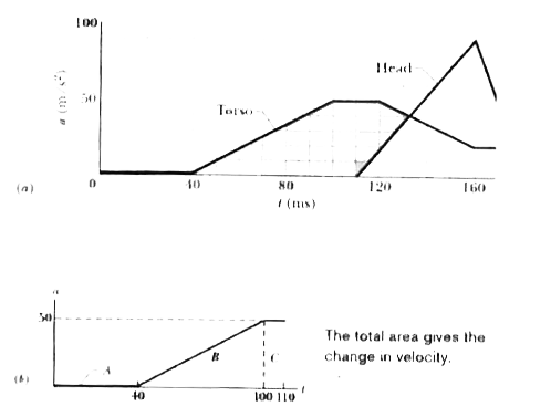
Gambar (a) $a-t$, kurva trapesium, $t_0$ dan $t_1$ diarsir di bawah kurva, “This area gives the change in velocity”.
Gambar (b) $v-t$, kurva trapezoid (dua garis di atas membentuk puncak, dinding kiri, tanpa dinding kanan), $t_0$ dan $t_1$ diarsir di bawah kurva, “This are gives the change in position”.
- Whether (a) and (b) are related, or just as illustration?
2-6 Graphical Integration in Motion Analysis (2 of 7) Link to heading
- Instantaneous velocity is defined as $\displaystyle v = \frac{dv}{dt}$
- In “calculus” language we would write $dx = vdt$, which we can integrate to obtaind: $$ dx = v(t)dt \rightarrow x(t_2) - x(t_1) = \sum v(t) \Delta t $$
- Graphically, this is adding up lots of small rectangles:
Gambar $v(t)$ pada grafik $v-t$ dengan daerah di bawah kurva dipartisi kotak-kotak.
$$ \Box + \Box + \dots + \Box + \Box = {\rm displacement} $$
$$ x(t_2) - x(t_1) = \int_{t_1}^{t_2} v(t) dt $$

2-6 Graphical Integration in Motion Analysis (3 of 7) Link to heading
- Integrating velocity:
- Given a graph of an object’s velocity $v$ versus time $t$, we can integrate to find position
- The Fundamental Theorem of Calculus gives: $$\tag{2-29} x_1 - x_0 = \int_{t_0}^{t_1} v dt $$
- The definite integral in the right can be evaluated from a graph: $$\tag{2-30} \int_{t_0}^{t_1} v dt = \left( \begin{array}{c} {\rm area \ between \ velocity \ curve} \newline {\rm and \ time \ axis, \ from} \ t_0 \ {\rm to} \ t_1 \end{array} \right) $$
2-6 Graphical Integration in Motion Analysis (4 of 7) Link to heading
- Integrating acceleration:
- Given a graph of an object’s acceleration $a$ versus time $t$, we can integrate to find velocity
- The Fundamental Theorem of Calculus gives: $$\tag{2-27} v_1 - v_0 = \int_{t_0}^{t_1} a dt $$
- The definite integral in the right can be evaluated from a graph: $$\tag{2-28} \int_{t_0}^{t_1} a dt = \left( \begin{array}{c} {\rm area \ between \ velocity \ curve} \newline {\rm and \ time \ axis, \ from} \ t_0 \ {\rm to} \ t_1 \end{array} \right) $$
2-6 Graphical Integration in Motion Analysis (5 of 7) Link to heading
url https://lowbackpain.com/news/what-is-whiplash-and-what-are-the-symptoms-of-severe-whiplash (2022)

Example
The graph shows the acceleration of a person’s head and torso in a whiplash incident.
Grafik (a) $a ({\rm m/s^2}) - t ({\rm ms})$, sumbu tegak (0, 50, 100), sumbu mendatar (0, 40, 80, 120, 160), kurva Torso: black (0, 0), (40, 0), (100, 50), (120, 50), (160, 20), (170, 20), kurva head: black (110, 0), (160, 90), (170, 50).
To calculate the torso speed at $t = 0.110 \ {\rm s}$ (assuming an initial speed of $0$), find the area under the pink curve:
Grafk (b) $a - t$, sumbu tegak (50), sumbu mendatar (40, 100, 110), kurva torso: pink (0, 0), (40, 0), (100, 50), (110, 50), region A, B, C, dashed line (0, 50) - (100, 50) - (100, 0).
- Area $A = 0$
- Area $B = 0.5 (0.060 \ {\rm s}) (50 \ {\rm m/s^2}) = 1.5 \ {\rm m/s}$
- Area $C = (0.010 \ {\rm s}) (50 \ {\rm m/s^2} = 0.5 \ {\rm m/s}$
- Total area = $2.0 \ {\rm m/s}$.
2-6 Graphical Integration in Motion Analysis (6 of 7) Link to heading
Example
A particle moves along the $x$-axis with varying velocity
Grafik $v \ ({\rm m \ s^{-1}}) - t \ ({\rm s})$, sumbu tegak (-10, 0, 10), sumbu mendatar (0, 2, 4, 6, 8), kurva: black (0, 10), (2, 0), (4, -10), (5, -10), (6, 0).
- a. Determine the average acceleration between t = 0 s to t = 4 s.
- b. Determine the instantaneous acceleration at t = 2 s and t = 4,5 s.
- c. Give a graphical sketch of the acceleration with respect to time.
- d. If at t = 0 s, the particle is at x = 2 m, determine its position at t = 6 s.
- e. What is the distance traveled by the particle between t = 0 s and t = 6 s.
2-6 Graphical Integration in Motion Analysis (7 of 7) Link to heading
Example
A particle moves along the $x$-axis and its position is given as a function of time by
$$ x(t) = (t^3 - 9t^2 + 24t) \ {\rm m} $$
- a. Determine the velocity and acceleration of the particle as a function of time t.
- b. Determine the values of t when the particle is at rest instantaneously.
- c. Determine the acceleration at these values of t.
- d. Determine the displacement of the particle between the time intervals 0 ≤ t ≤ 2 and 0 ≤ t ≤ 4
- e. Determine the distance traveled by the particle between the time interval 0 ≤ t ≤ 4
Summary (1 of 5) Link to heading
Position
- Relative to origin
- Positive and negative directions
Displacement
- Change in position (vector) $$\tag{2-1} \Delta x = x_2 - x_1 $$
Summary (1 of 5) Link to heading
Average Velocity
- $\displaystyle \frac{ {\rm Displacement \ (vector)} }{ {\rm time} }$ $$\tag{2-2} v_{\rm avg} = \frac{\Delta x}{\Delta t} = \frac{x_2 - x_1}{t_2 - t_1} $$
Average speed
- $\displaystyle \frac{ {\rm Distance \ traveled} }{ {\rm time} }$
$$\tag{2-3} s_{\rm avg} = \frac{\rm total \ distance}{\Delta t} $$
Summary (3 of 5) Link to heading
Instantaneous Velocity
- At a moment in time
- Speed is its magnitude $$\tag{2-4} v = \lim_{\Delta t \to 0} \frac{\Delta x}{\Delta t} = \frac{dx}{dt} $$
Average acceleration
- Ratio of change in velocity to change in time
$$\tag{2-7} a_{\rm avg} = \frac{v_2 - v_1}{t_2 - t_1} = \frac{\Delta v}{\Delta t} $$
Summary (4 of 5) Link to heading
Instantaneous acceleration
- First derivative of velocity
- Second derivative of position $$\tag{2-8} a = \frac{dv}{dt} $$
Summary (5 of 5) Link to heading
Constant acceleration
- Includes free-fall, where $a = -g$ along the vertical axis
| Equation Number | Equation | Missing quantity |
|---|---|---|
| 2-11 | $v = v_0 + at$ | $x - x_0$ |
| 2-15 | $x - x_0 = v_0 t + \frac12 at^2$ | $v$ |
| 2-16 | $v^2 = v_0^2 + 2a(x - x_0)$ | $t$ |
| 2-17 | $x - x_0 = \frac12 (v_0 + v) t$ | $a$ |
| 2-18 | $x - x_0 = vt - \frac12 at^2$ | $v_0$ |
Table (2-1)
Assignment-01 Link to heading
- Check your presense on SIX.
- Create Medium account for this course.
- Create GitHub account for this course.
- Fork related GitHub repository to this course
- Report the results in an issue of related GitHub repository
- Report your username for Medium and GitHub, and link to forked repository to the issue and also in Edunex.
Copyright Link to heading
Copyright © 2018 John Wiley & Sons, Inc.
All rights reserved. Reproduction or translation of this work beyond that permitted in Section 117 of the 1976 United States Act without the express written permission of the copyright owner is unlawful. Request for further information should be addressed to the Permissions Department, John Wiley & Sons, Inc. The purchaser may make back-up copies for his/her own use only and not for distribution or resale. The Publisher assumes no responsibility for errors, omissions, or damages, caused by the use of these programs or from the use of the information contained herein.
C. SECTION 117 COMPUTER PROGRAM EXEMPTIONS Link to heading
Section 117 of the Copyright Act of 1976 was enacted in the Computer Software Copyright Amendments of 1980 in response to the recommendations of the National Commission on New Technological Uses of Copyrighted Works’ (CONTU). Section 117 permits the owner of a copy of a computer program to make an additional copy of the program for purely archival purposes if all archival copies are destroyed in the event that continued possession of the computer program should cease to be rightful, or where the making of such a copy is an essential step in the utilization of the computer program in conjunction with a machine and that it is used in no other manner.